Autoencoder
Wiki: https://en.wikipedia.org/wiki/Autoencoder
Code source: https://github.com/aymericdamien/TensorFlow-Examples/blob/master/examples/3_NeuralNetworks/autoencoder.py
MNIST Dataset: http://yann.lecun.com/exdb/mnist/
References: Y. LeCun, L. Bottou, Y. Bengio, and P. Haffner. "Gradient-based learning applied to document recognition." Proceedings of the IEEE, 86(11):2278-2324, November 1998.
Introduction
An autoencoder is a type of artificial neural network used to learn efficient data codings in an unsupervised manner. The aim of an autoencoder is to learn a representation (encoding) for a set of data, typically for dimensionality reduction, by training the network to ignore signal “noise”. Along with the reduction side, a reconstructing side is learnt, where the autoencoder tries to generate from the reduced encoding a representation as close as possible to its original input, hence its name. Several variants exist to the basic model, with the aim of forcing the learned representations of the input to assume useful properties.
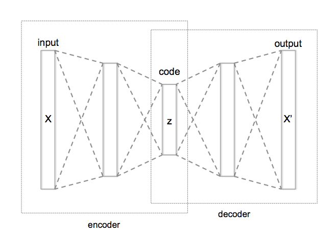
Structure
An autoencoder consists of two parts, the encoder and the decoder, which can be defined as transitions $\phi$ and $\psi$, such that:
$$\phi: x \rightarrow h, h = \phi(x)$$$$\psi: h \rightarrow \tilde{x}, \tilde{x} = \psi (h)$$$$\phi ,\psi ={\underset{\phi ,\psi }{\operatorname {arg\,min} }}\,\sum_{i=1}^N ||x_i - \psi (\phi (x_i)) ||^2$$In the simplest case, $$ h =\sigma (Wx + b)$$
Embedding $h$ is usually referred to as code, latent variables, or latent representation. Here, $\sigma$ is an element-wise activation function such as a sigmoid function or a rectified linear unit. $W$ is a weight matrix and $b$ is a bias vector. Weights and biases are usually initialized randomly, and then updated iteratively during training through Backpropagation. After that, the decoder stage of the autoencoder maps $h$ to the reconstruction $\tilde{x}$ of the same shape as $x$:
$$\tilde{x} = \sigma (\tilde{W}h +\tilde{b})$$where $\tilde{W}$, $\tilde{b}$ for the decoder may be unrelated to the corresponding $W$, $b$ for the encoder.
Autoencoders are trained to minimise reconstruction errors (such as squared errors), often referred to as the "loss": $$L(X, \tilde{X})=\sum_{i=1}^N||x_i -\tilde{x}_i||^2$$
As mentioned before, the training of an autoencoder is performed through Backpropagation of the error, just like a regular feedforward neural network.
import tensorflow as tf
import numpy as np
import matplotlib.pyplot as plt
import pandas as pd

# Import MNIST data
mnist_train = pd.read_csv("../input/mnist-in-csv/mnist_train.csv")
mnist_test = pd.read_csv("../input/mnist-in-csv/mnist_test.csv")
x_train = np.array(mnist_train.iloc[:, 1:]).reshape(-1, 28*28) / 255
# y_train = np.array(mnist_train.iloc[:, 0])
x_test = np.array(mnist_test.iloc[:, 1:]).reshape(-1, 28*28) / 255
# y_test = np.array(mnist_test.iloc[:, 0])
n_train_samples = x_train.shape[0]

# Network Parameters
num_hidden_1 = 256 # 1st layer num features
num_hidden_2 = 128 # 2nd layer num features (the latent dim)
num_input = 784 # MNIST data input (img shape: 28*28)

# tf Graph input (only pictures)
X = tf.placeholder("float", [None, num_input])

weights = {
    'encoder_h1': tf.Variable(tf.random_normal([num_input, num_hidden_1])),
    'encoder_h2': tf.Variable(tf.random_normal([num_hidden_1, num_hidden_2])),
    'decoder_h1': tf.Variable(tf.random_normal([num_hidden_2, num_hidden_1])),
    'decoder_h2': tf.Variable(tf.random_normal([num_hidden_1, num_input])),
}
biases = {
    'encoder_b1': tf.Variable(tf.random_normal([num_hidden_1])),
    'encoder_b2': tf.Variable(tf.random_normal([num_hidden_2])),
    'decoder_b1': tf.Variable(tf.random_normal([num_hidden_1])),
    'decoder_b2': tf.Variable(tf.random_normal([num_input])),
}

# Building the encoder
def encoder(x):
    # Encoder Hidden layer with sigmoid activation #1
    layer_1 = tf.nn.sigmoid(tf.add(tf.matmul(x, weights['encoder_h1']), biases['encoder_b1']))
    # layer_1 = tf.nn.relu(tf.add(tf.matmul(x, weights['encoder_h1']), biases['encoder_b1']))

    # Encoder Hidden layer with sigmoid activation #2
    layer_2 = tf.nn.sigmoid(tf.add(tf.matmul(layer_1, weights['encoder_h2']), biases['encoder_b2']))
    return layer_2

# Building the decoder
def decoder(x):
    # Decoder Hidden layer with sigmoid activation #1
    layer_1 = tf.nn.sigmoid(tf.add(tf.matmul(x, weights['decoder_h1']), biases['decoder_b1']))
    # layer_1 = tf.nn.relu(tf.add(tf.matmul(x, weights['decoder_h1']), biases['decoder_b1']))

    # Decoder Hidden layer with sigmoid activation #2
    layer_2 = tf.nn.sigmoid(tf.add(tf.matmul(layer_1, weights['decoder_h2']), biases['decoder_b2']))
    return layer_2

# Construct model
embedding = encoder(X)
recon_x = decoder(embedding)

# Prediction
y_pred = recon_x
# Targets (Labels) are the input data.
y_true = X

# Define loss and optimizer, minimize the squared error
loss = tf.reduce_mean(tf.pow(y_true - y_pred, 2))
learning_rate = tf.placeholder("float32")
optimizer = tf.train.RMSPropOptimizer(learning_rate).minimize(loss)

print('Autoencoder is constructed.')
RMSProp: https://en.wikipedia.org/wiki/Stochastic_gradient_descent#RMSProp
RMSProp (for Root Mean Square Propagation) is also a method in which the learning rate is adapted for each of the parameters. The idea is to divide the learning rate for a weight by a running average of the magnitudes of recent gradients for that weight. So, first the running average is calculated in terms of means square, $$v(w,t):=\gamma v(w,t-1)+(1-\gamma )(\nabla Q_{i}(w))^{2}$$ where, $\gamma$ is the forgetting factor.
And the parameters are updated as,
$$w:=w-{\frac {\eta }{\sqrt {v(w,t)}}}\nabla Q_{i}(w)$$RMSProp has shown excellent adaptation of learning rate in different applications. RMSProp can be seen as a generalization of Rprop and is capable to work with mini-batches as well opposed to only full-batches.
# Training Parameters
learning_rate_AE = 0.01
max_epoch = 10000
# max_epoch = 50000
batch_size = 256

display_step = 1000

# Start Training
# Start a new TF session
with tf.Session() as sess:
    # Initialize the variables (i.e. assign their default value)
    sess.run(tf.global_variables_initializer())

    # Training
    for i in range(max_epoch):
        # Prepare a batch
        tmp_index = np.random.permutation(n_train_samples)
        batch_x = x_train[tmp_index[:batch_size], :]
        # Run optimization op (backprop) and cost op (to get loss value)
        _, l = sess.run([optimizer, loss], feed_dict={X:batch_x, learning_rate:learning_rate_AE})
        # Display logs per step
        if i % display_step == 0:
            print('Step %i: Minibatch Loss: %f' % (i, l))

    # Testing
    # Encode and decode images from test set and visualize their reconstruction.
    n = 4
    img_orig = np.empty((28 * n, 28 * n))
    img_recon = np.empty((28 * n, 28 * n))
    for i in range(n):
        # MNIST test set
        batch_x = x_test[i*n:(i+1)*n, :]
        # Encode and decode the digit image
        g = sess.run(recon_x, feed_dict={X:batch_x})

        # Display original images
        for j in range(n):
            # Draw the original digits
            img_orig[i * 28:(i + 1) * 28, j * 28:(j + 1) * 28] = batch_x[j].reshape([28, 28])
        # Display reconstructed images
        for j in range(n):
            # Draw the reconstructed digits
            img_recon[i * 28:(i + 1) * 28, j * 28:(j + 1) * 28] = g[j].reshape([28, 28])

    print("Original Images")
    plt.figure(figsize=(n, n))
    plt.imshow(img_orig, origin="upper", cmap="gray")
    plt.show()

    print("Reconstructed Images")
    plt.figure(figsize=(n, n))
    plt.imshow(img_recon, origin="upper", cmap="gray")
    plt.show()

